
The audio examples on this page are part of the course Spatial Audio – Practical Master Guide. They also accompany this document:
Jens Ahrens, “Introduction to Ambisonics, Part 1: The Part With No Math,” Technical Report v. 1.0, Chalmers University of Technology, 2025 [pdf]
as well as this video series.
We obtained the source signals for the audio examples from here.
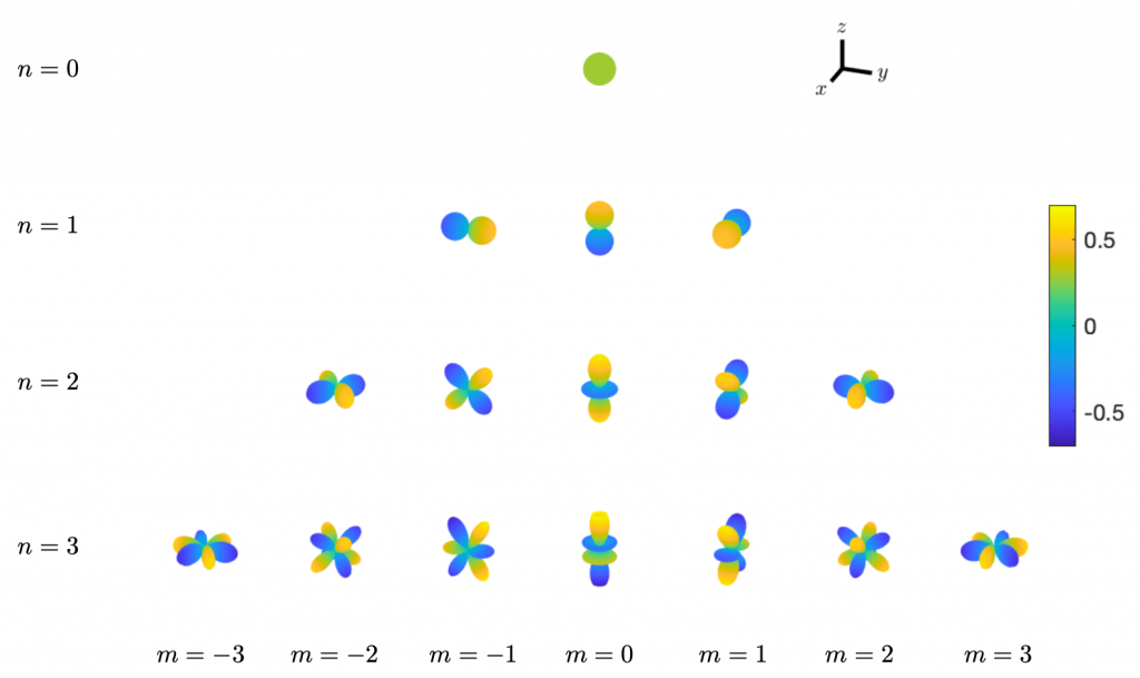
Below is an illustration of the spherical harmonics for the orders n = 0, 1, 2, 3. These shapes also correspond to the directivities that a theoretical microphone would need to have for recording the given channel of the ambisonic signal.
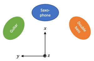
The audio examples allow you to listen to the individual channels of an ambisonic signal that represents the following scenario (which includes also a bit of reverberation):
The ambisonic signal is computer generated. We obtained the source signals from here.
The channels are sorted according to ACN (ambisonic channel number), i.e. the channels walk through the spherical harmonic modes as arranged in the above table starting from the top and walking through each row from left to right.
| Channel | Mode (n,m) | Audio signal |
| 1 | (0, 0) | |
| 2 | (1, -1) | |
| 3 | (1, 0) | |
| 4 | (1, 1) | |
| 5 | (2, -2) | |
| 6 | (2, -1) | |
| 7 | (2, 0) | |
| 8 | (2, 1) | |
| 9 | (2, 2) |
The following audio examples are binaural renderings of computer-generated ambisonic signals of different orders N. The differences between different orders tend to be more obvious when head tracking is applied, which is unfortunately not possible here. You will hear the same music like above circling around your head instead to achieve similar spatial dynamics like with head tracking. All instruments are colocated in these examples to make the differences easier to identify. The examples labelled Equalized are rendered with magLS.
Focus, for example, on how well the low-frequency content is localizable at the different orders.
| Ambisonic order N | Unequalized | Equalized |
| 0 | ||
| 1 | ||
| 5 | ||
| 7 |
Acknowledgments
This work received funding under the Erasmus+ programme of the European Commission und grant 2022-1-PL01-KA220-VET-000085305.